In this post we are going to discuss the S&P 500 Exponential GARCH Asset Volatility model. The volatility model that we will develop in this post for S&P 500 can also be used for other indices like Dow Jones, Nasdaq, FTSE 100, DAX , CAC 40, Hang Seng etc as well as stocks like Apple, Google, Facebook etc. There are many day traders who love to trade S&P 500 index as well as the other stock indices that have been mentioned above. Did you read the book How To Make More Money Than God-Hedge Funds and Making of New Elite? Asset volatility is an important subject in quantitative finance as it has got very important applications. If you want a job as a quant at a hedge fund than you should know in intimate detail the different asset volatility models. The most important application of asset volatility models is in options pricing. Most hedge funds love to trade options. Asset volatility models are also very important in calculating Value at Risk for managing the risk of a portfolio. Most hedge funds use this Value at Risk measure a lot in quantifying the risk to their asset portfolio.
You should read this post if you are thinking of becoming an options trader. This is something very important for you to understand. We talk of asset volatility most of the the time. But we cannot observe it directly. We can only observe the price of the asset and its derivative which will most of the time be options. So you should keep this in mind We cannot measure asset volatility directly. We can only calculate it or to be more precise estimate it with the price of the asset and the options contract on that asset. Read this post on how to develop your artificial intelligence machine learning stock trading system.
The first asset volatility model was the Autoregressive Conditional Heteroscedastic ARCH Model. This model had some limitations so the General Autoregressive Conditional Heteroscedastic GARCH Model was developed. You should read this post that explains the ARIMA and GARCH models. Most of the time you will hear about the GARCH model. In this post however we will talk of a modification of this GARCH model which is known as the Exponential GARCH model.The exponential GARCH model is also known as the EGARCH model. There are many more asset volatility models that have been developed that includes IGARCH, TGARCH and NGARCH.
Characterisitics of Asset Volatility
Now as said above we cannot observe volatility directly. But we can observe some of its characteristics. The most important ones are the volatility clusters. Volatility clusters is a characteristic that means volatility is high for some periods of time and low for other periods of time. You can observe this thing at the time of economic news release when the currencies and stocks become highly volatility. This high volatility lasts for sometime. The stocks become volatile when there is an important announcement by the FED. This volatility persists for sometime. Market tries to absorb the new information which is the reason for this high volatility. FOMC Meeting minutes release time is when stock market can become highly volatile. Now quantitative finance revolves around return and volatility. Read this post on how to predict stock return using support vector machines.
The second think that you should know is the there are no volatility jumps.Volatility evolves over time in a continuous manner. It is not like that suddenly the market becomes highly volatile. So there are no volatility jumps.Thirdly volatility cannot become infinite. Volatility stays within a certain range. Now this is something important for you to understand.Volatility reacts differently to a big price increase as compared to a big price decrease. Big price drop has a much higher volatility as compared to a big price increase. ARCH and GARCH models cannot cater for this leverage effect. ARCH and GARCH have the same volatility for the big price increase as well as big price decrease. Due to this reason EGARCH and TGARCH models were developed as they introduce an asymmetric behavior in asset volatility. As said before we cannot observe volatility directly. We cannot only estimate it with the stock price and the options contract prices on that stock. Before we continue there are three types of volatility that we can calculate.
We will be using R in doing the modelling. R is a powerful data science scripting language that is very popular with the quants. You should have R and RStudio installed on your computer. You should master R if you want to become a quant. Read this post on how to do algorithmic trading with R. When it comes to time series analysis R is very powerful. Python cannot beat R when it comes to time series analysis.
Types of Volatility Measures
There are three types of volatility measure that we use:
1. Volatility as condition standard deviation of the stock daily returns. This is what we will estimate in this post. Volatility of a stock return is estimated on an annualized basis. Since there are 252 trading days in a year we can calculate the annualized volatility by multiplying the daily volatility by sqr(252) where sqr is the square root.
2. Implied volatility is estimated through the stock options pricing formula like the Black Scholes. You should read this post in which I have posted videos that explain this Black Scholes formula in detail. Read this post as it discusses how this formula is derived, what are the assumptions made while deriving the formula and what are the limitations. Since it is formula dependent there are certain limitations to this approach of calculating the implied volatility. You can read this post in which I have given the python code for calculating Black Scholes Options Pricing formula.
3. We can also calculate daily volatility from the high frequency trading data intraday returns. For example we can use the 5 minute time interval to estimate the daily volatility. This is known as Realized Volatility. In the next post we can discuss in detail how we are going to calculate the realized volatility from the high frequency trading data.
S&P 500 eGARCH(2,1) Volatility Model Using rugarch R package
This is how we are going to build the model. First we need to download S&P 500 daily price data from Yahoo Finance.
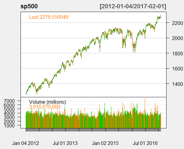
> #load library
> library(quantmod)
> #create an environment
> SP500 <- new.env()
> #first we download the daily time series data from Yahoo Finance
> getSymbols("^GSPC", env = SP500, src = "yahoo",
+            from = as.Date("2012-01-04"), to = as.Date("2017-02-01"))
[1] "GSPC"
> sp500 <- SP500$GSPC
> head(sp500)
           GSPC.Open GSPC.High GSPC.Low GSPC.Close GSPC.Volume GSPC.Adjusted
2012-01-04   1277.03   1278.73  1268.10    1277.30  3592580000       1277.30
2012-01-05   1277.30   1283.05  1265.26    1281.06  4315950000       1281.06
2012-01-06   1280.93   1281.84  1273.34    1277.81  3656830000       1277.81
2012-01-09   1277.83   1281.99  1274.55    1280.70  3371600000       1280.70
2012-01-10   1280.77   1296.46  1280.77    1292.08  4221960000       1292.08
2012-01-11   1292.02   1293.80  1285.41    1292.48  3968120000       1292.48
> class(sp500)
[1] "xts" "zoo"
> dim(sp500)
[1] 1278    6
> # Plot the daily price series and volume
> chartSeries(sp500,theme="white")
Below is the plot for the S&P 500 daily time series.
Now we take the Box Ljung test of the daily log returns of S&P 500 daily time series of the closing price.
> #calculate the log returns
> #calculate the log returns
> sp500lr <-log(sp500$GSPC.Close+1)
> #Box Ljung Test for serial correlation of log returns
> Box.test(sp500lr,lag=1,type="Ljung")

	Box-Ljung test

data:  sp500lr
X-squared = 1271.6, df = 1, p-value < 2.2e-16
You can see from the above Box Ljung test that the daily log returns of S&P 500 daily time series are not serially correlated. Now we will be using rugarch package. This is a powerful package. You should practice with this R package a lot if you are planning to calculate the volatility of stock indices on a daily basis. You can download rugarch package 107 page PDF from R cran site. It contains full details on the different methods that you can call using this package. We can model different types of GARCH models with this package. First we load this package than we create spec.
> #load rugarch library
> library(rugarch)
>
> #Fit the EGARCH model
>
> # create a cluster object to be used as part of this demonstration
> cluster <- makePSOCKcluster(15)
> #ask R to show specs
> spec <- ugarchspec()
> show(spec)

*---------------------------------*
*       GARCH Model Spec          *
*---------------------------------*

Conditional Variance Dynamics
------------------------------------
GARCH Model		: sGARCH(1,1)
Variance Targeting	: FALSE

Conditional Mean Dynamics
------------------------------------
Mean Model		: ARFIMA(1,0,1)
Include Mean		: TRUE
GARCH-in-Mean		: FALSE

Conditional Distribution
------------------------------------
Distribution	:  norm
Includes Skew	:  FALSE
Includes Shape	:  FALSE
Includes Lambda	:  FALSE
You can see from above that the package is suggesting a standard GARCH(1,1) package with ARFIMA(1,0,1). Let’s see how many models that are possible.
> #number of possible models
> nrow(expand.grid(GARCH = 1:14, VEX = 0:1, VT = 0:1,
+                  Mean = 0:1, ARCHM = 0:2,
+                  ARFIMA = 0:1, MEX = 0:1, DISTR = 1:10))
[1] 13440
You can see with the above specifications there are 13440 models that we can fit. Below we fit a eGARCH model with order(2,1) meaning it is second order autoregressive and first order moving average. Most of the time order(1,1) is sufficient for modelling purpose. Since this is a post meant for training and exploration, we choose order(2,1).
> #fit the rugarch eGarch model with student t distribution
> spec = ugarchspec(variance.model = list(model = 'eGARCH',
+                                         garchOrder = c(2, 1)),
+                   distribution = 'std')
> setstart(spec) <- list(shape = 5)
> egarch1<- ugarchfit(spec, sp500lr[1:1000, , drop = FALSE], solver = 'hybrid')
> egarch1

*---------------------------------*
*          GARCH Model Fit        *
*---------------------------------*

Conditional Variance Dynamics
-----------------------------------
GARCH Model	: eGARCH(2,1)
Mean Model	: ARFIMA(1,0,1)
Distribution	: std

Optimal Parameters
------------------------------------
        Estimate  Std. Error     t value Pr(>|t|)
mu      7.153286    0.012530  5.7091e+02 0.000000
ar1     0.999666    0.000000  4.0443e+07 0.000000
ma1     0.000532    0.025793  2.0638e-02 0.983535
omega  -0.938738    0.006589 -1.4247e+02 0.000000
alpha1 -0.396606    0.024005 -1.6522e+01 0.000000
alpha2  0.051018    0.024828  2.0548e+00 0.039897
beta1   0.902905    0.000105  8.5776e+03 0.000000
gamma1 -0.064610    0.054744 -1.1802e+00 0.237911
gamma2  0.131327    0.046940  2.7978e+00 0.005145
shape  13.351651    4.896861  2.7266e+00 0.006400

Robust Standard Errors:
        Estimate  Std. Error     t value Pr(>|t|)
mu      7.153286    0.001466  4.8796e+03 0.000000
ar1     0.999666    0.000000  3.3707e+07 0.000000
ma1     0.000532    0.023802  2.2364e-02 0.982158
omega  -0.938738    0.006467 -1.4516e+02 0.000000
alpha1 -0.396606    0.021293 -1.8626e+01 0.000000
alpha2  0.051018    0.023691  2.1535e+00 0.031280
beta1   0.902905    0.000105  8.5584e+03 0.000000
gamma1 -0.064610    0.053296 -1.2123e+00 0.225408
gamma2  0.131327    0.046005  2.8546e+00 0.004309
shape  13.351651    4.401599  3.0334e+00 0.002418

LogLikelihood : 3527.377

Information Criteria
------------------------------------

Akaike       -7.0348
Bayes        -6.9857
Shibata      -7.0350
Hannan-Quinn -7.0161

Weighted Ljung-Box Test on Standardized Residuals
------------------------------------
                        statistic p-value
Lag[1]                     0.1285  0.7200
Lag[2*(p+q)+(p+q)-1][5]    1.6689  0.9931
Lag[4*(p+q)+(p+q)-1][9]    3.7400  0.7503
d.o.f=2
H0 : No serial correlation

Weighted Ljung-Box Test on Standardized Squared Residuals
------------------------------------
                         statistic p-value
Lag[1]                       0.021  0.8848
Lag[2*(p+q)+(p+q)-1][8]      2.104  0.8425
Lag[4*(p+q)+(p+q)-1][14]     5.127  0.7536
d.o.f=3

Weighted ARCH LM Tests
------------------------------------
            Statistic Shape Scale P-Value
ARCH Lag[4]     1.065 0.500 2.000  0.3021
ARCH Lag[6]     1.963 1.461 1.711  0.4990
ARCH Lag[8]     4.395 2.368 1.583  0.3205

Nyblom stability test
------------------------------------
Joint Statistic:  2.5149
Individual Statistics:
mu     0.5614
ar1    0.1489
ma1    0.1131
omega  0.2158
alpha1 0.4151
alpha2 0.3839
beta1  0.2224
gamma1 0.5211
gamma2 0.3963
shape  0.3781

Asymptotic Critical Values (10% 5% 1%)
Joint Statistic:     	 2.29 2.54 3.05
Individual Statistic:	 0.35 0.47 0.75

Sign Bias Test
------------------------------------
                   t-value    prob sig
Sign Bias            1.975 0.04850  **
Negative Sign Bias   1.512 0.13092
Positive Sign Bias   1.749 0.08066   *
Joint Effect         5.516 0.13767


Adjusted Pearson Goodness-of-Fit Test:
------------------------------------
  group statistic p-value(g-1)
1    20     48.96    0.0001861
2    30     59.90    0.0006356
3    40     69.84    0.0017471
4    50     71.60    0.0192722


Elapsed time : 24.87401
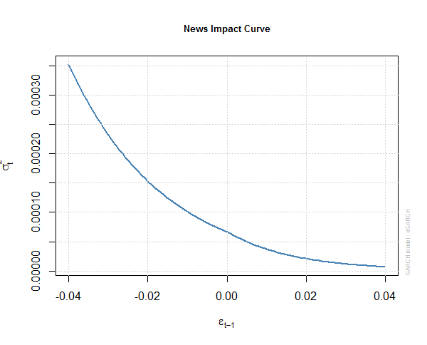
Above you can see the full details of the eGARCH(2,1) model that we have fitted to S&P 500 daily log return series. R took around 25 seconds to do all the calculations which is pretty fast. Below are some plots of this eGARCH(2,1) model. This is the news impact curve for the egarch1 model.
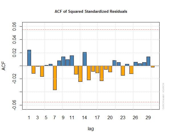
This is the auto correlation function of the squared standardized residuals of egarch1.
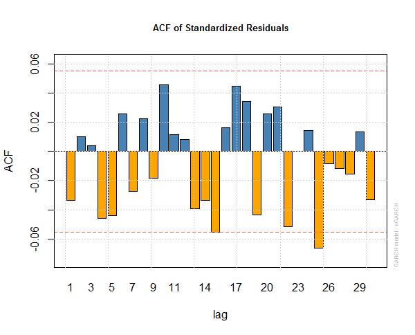
This is the auto correlation function plot of standardized residuals of egarch1 model.
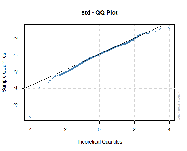
This is the standard QQ plot of the residuals of egarch1. You can see the residuals are still flat tailed and not strictly normal, So our egarch1 model may not be very good.
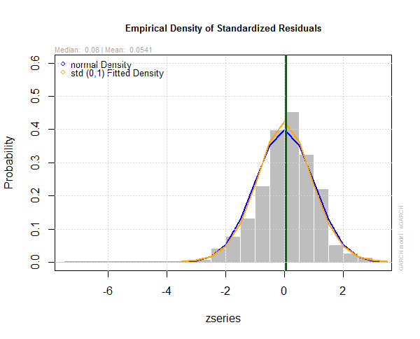
This is the plot of the empirical density of the standardized residuals of egarch1 model.
We try to build 2 more models as more streaming data comes in.
> spec <-getspec(egarch1)
> setfixed(spec) <- as.list(coef(egarch1))
> #filter new data that has streamed in
> egarch2 <- ugarchfilter(spec, sp500lr[1:1250, ], n.old = 1000)
> egarch3 <- ugarchfilter(spec, sp500lr[1001:1250, ])
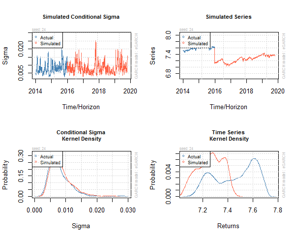
Now we can also do simulation on our fitted egarch1 model.
> #simulating GARCH models
> sim <- ugarchsim(egarch1, n.sim = 1000, m.sim = 25, rseed = 1:25)
> show(sim)

*------------------------------------*
*       GARCH Model Simulation       *
*------------------------------------*
Model : eGARCH
Horizon:  1000
Simulations: 25
              Seed Sigma2.Mean Sigma2.Min Sigma2.Max Series.Mean Series.Min
sim1             1    9.13e-05   5.97e-06   0.000964        7.27       7.04
sim2             2    9.24e-05   5.25e-06   0.000646        7.05       6.86
sim3             3    9.84e-05   3.39e-06   0.001159        7.01       6.85
sim4             4    8.90e-05   9.27e-06   0.000599        7.06       6.96
sim5             5    8.42e-05   3.01e-06   0.000666        7.06       6.86
sim6             6    9.08e-05   3.60e-06   0.000782        7.16       7.00
sim7             7    8.90e-05   2.42e-06   0.001390        7.20       6.89
sim8             8    8.36e-05   5.22e-06   0.000903        7.30       7.06
sim9             9    7.44e-05   6.62e-06   0.000446        7.35       7.13
sim10           10    1.00e-04   6.28e-06   0.001035        7.22       6.81
sim11           11    9.40e-05   6.81e-06   0.000688        6.98       6.76
sim12           12    7.96e-05   4.16e-06   0.000845        7.21       7.02
sim13           13    7.70e-05   4.42e-06   0.000658        7.21       6.99
sim14           14    1.03e-04   4.41e-06   0.000839        7.04       6.77
sim15           15    7.82e-05   3.96e-06   0.000768        7.40       7.15
sim16           16    8.41e-05   2.65e-06   0.001233        7.27       7.04
sim17           17    7.57e-05   1.89e-06   0.000778        7.36       7.07
sim18           18    1.20e-04   6.17e-06   0.002533        6.94       6.54
sim19           19    9.14e-05   3.87e-06   0.001020        7.04       6.88
sim20           20    8.09e-05   4.41e-06   0.000627        7.25       7.07
sim21           21    7.24e-05   3.16e-06   0.000532        7.31       7.03
sim22           22    9.12e-05   6.72e-06   0.000951        7.12       6.86
sim23           23    1.01e-04   5.22e-06   0.000879        7.08       6.83
sim24           24    7.90e-05   8.37e-06   0.000641        7.26       7.04
sim25           25    9.80e-05   4.06e-06   0.001675        7.21       6.85
Mean(All)        0    8.87e-05   4.85e-06   0.000930        7.17       6.93
Actual           0    6.83e-05   4.69e-06   0.000782        7.46       7.15
Unconditional    0    6.33e-05         NA         NA        7.15         NA
              Series.Max
sim1                7.50
sim2                7.29
sim3                7.16
sim4                7.18
sim5                7.27
sim6                7.28
sim7                7.38
sim8                7.50
sim9                7.50
sim10               7.42
sim11               7.19
sim12               7.40
sim13               7.39
sim14               7.23
sim15               7.58
sim16               7.48
sim17               7.56
sim18               7.18
sim19               7.18
sim20               7.45
sim21               7.55
sim22               7.37
sim23               7.32
sim24               7.45
sim25               7.42
Mean(All)           7.37
Actual              7.66
Unconditional         NA
Below is the plot of this simulation.
We can do forecasting as well. Volatility calculations are very important in options price calculations. In a future post I will show you how we are going to use our volatility model in pricing an options contract. Now this was a short introduction to how to make volatility models for stock indices like S&P 500. I have developed a few courses on R that you can take a look at. First course is R for Traders. In this course I give you an introduction to how you are going to use R for statistical analysis that you can use in your trading. The second course is Machine Learning Using R for Traders. In this course I build upon the first course R for Traders. I explains some important machine learning algorithms and then show you how to build predictive models using those machine learning algorithms using R. The third course is Algorithmic Trading With R. This course build upon the first 2 courses. I show you how we are going to build algorithmic trading systems using R and APIs provided by brokers.