If you are an options trader, you should read this post. In this post we give you a short few lines python code that you can use to calculate the option price using the Black Scholes Options Pricing Formula. If you are not familiar with Black Scholes Options Pricing Formula, you should watch these videos. These videos explain the derivation of Black Scholes formula in simple terms. Watch these videos. In these videos the instructor derives Black Scholes formula mathematically. Once you have understood the mathematical formula and how it is used to calculate the call option price as well as put option price. You just need to plugin the values in the formula and calculate the price.
Now lets start. First you need to install Python on your computer. This can be easily done. Just visit the Python official website. Download the version of Python suitable for your computer depending on whether you have a Windows, Mac, Linux etc. Once you have installed Python on your computer you are all set to easily calculate the option price. We need the following inputs before we can calculate option price.
–>Current stock price S
–>Exercise price X
–>Maturity in years T
–>Continuously compounded risk free rate r
–>Volatility of the underlying stock sigma
Below is the python code for calculating the price of the option contract.
from math import *

#first define these 2 functions
def d1(S,X,T,r,sigma):
    return (log(S/X)+(r+sigma*sigma/2.)*T)/(sigma*sqrt(T))

def d2(S,X,T,r,sigma):
    return d1(S,X,T,r,sigma)-sigma*sqrt(T)

#define the call option price function
def bs_call(S,X,T,r,sigma):
     return S*CND(d1(S,X,T,r,sigma))-X*exp(-r*T)*CND(d2(S,X,T,r,sigma))

#define the put options price function
def bs_put(S,X,T,r,sigma):
      return X*exp(-r*T)-S + bs_call(S,X,T,r,sigma)

#define cumulative standard normal distribution
def CND(X):
     (a1,a2,a3,a4,a5)=(0.31938153,-0.356563782,1.781477937,-1.821255978,1.330274429)
     L = abs(X)
     K=1.0/(1.0+0.2316419*L)
     w=1.0-1.0/sqrt(2*pi)*exp(-L*L/2.)*(a1*K+a2*K*K+a3*pow(K,3)+a4*pow(K,4)+a5*pow(K,5))
     if X<0:
        w=1.0-w
     return w
I have pasted the above python code. You will need to indent the above code.Let’s run this code now. Let’s calculate the call options price.
>>> bs_call(40,42,0.5,0.1,0.2)
2.2777859030683096
Now let’s calculate the put option price
>>> bs_put(40,35,0.5,0.1,0.2)
0.23567541070870845
This is it. Now the problem with the Black Scholes options price formula is that it makes a few simplifying assumptions that don’t work in reality. The first assumption is that market is efficient. Market efficient means information instantaneously gets reflected in the stock price. This assumption does not hold in reality. Information about a stock slowly diffuses through the market. This is what is considered to be true. Markets are inefficient in the short run. But over the long run, markets are efficient. The second assumption of stock returns are normally distributed. This assumption is not good. In reality it has been shown that stock returns are long tailed and skewed.
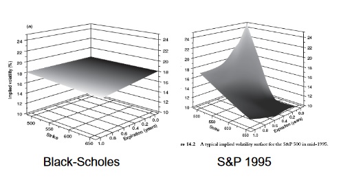
Black Scholes formula assumes that the volatility is independent of strike price and maturity. This means that the implied volatility should be a flat plane. Prior to 1987 stock market crash this was indeed the case. Surprisingly now the market has changed and implied volatility of an options contract now depends on strike price and time to expiry. Due to this reason Black Scholes formula cannot explain the volatility smile phenomenon. Volatility smile is not predicted at all by this formula. Below is a graph that explains what this phenomenon is. According to Black Scholes formula, implied volatility should be flat. But it it not.
After making the modifications in the above assumptions, quants have been able to derive a modified Black Scholes formula that works most of the time. For a beginner, you can assume that this formula work. We have provided you with the python code. You can use it. Today quantitative models are increasingly being used in trading. If you are solely using technical analysis than you must have understood by now. Things are not working. Start your journey into quantitative trading. You will need to learn probability and statistics, artificial intelligence and machine learning. The journey looks difficult but it is worth taking. Did you check our course Machine Learning Using R For Traders? In this course we teach you how to use R in machine learning. R is a powerful data science and machine learning language just like Python. You should learn both Python and R. If you don’t know R, then you should first try our R For Traders course.